Table of Input and Output;
| Variable units of labour | Fixed Assets (Hecteres of Land) | Total Product (kg) | Average Product (kg) | Marginal product (kg) |
| 1 | 3 | 8 | 8 | - |
| 2 | 3 | 18 | 9 | 10 |
| 3 | 3 | 36 | P | 18 |
| 4 | 3 | 48 | 12 | 12 |
| 5 | 3 | 55 | 11 | 7 |
| 6 | 3 | 60 | Q | 5 |
| 7 | 3 | 60 | 8.6 | S |
| 8 | 3 | 56 | 7 | T |
Use the table to answer the following questions:
(a) Complete table by calculating the missing figures P, Q, R, S, T.
(b) Draw the Total Product (TP) and Marginal Product (MP) curve in one diagram. (No graph sheet is required).
(c) Explain the relationship between TP and MP.


(a)(i) Total product = Average product x Units of labour
36 = P x 3, P3 = 36 P = 36
P= \(\frac{36}{3}\) = 12
(ii) Q = Total product = \(\frac{60}{6} = 10
Labour
(iii) R = \(\frac{48-36}{4-3}\)
\(\frac{12}{12}\) = 1
(iv) S = \(\frac{60 - 60}{6 - 5} = \frac{0}{1}\) = 0
(v) T = \(\frac{56 - 60}{8 - 7}\) = \frac{-4}{1}\) = -4
| Variable units of labour | Fixed Assets (Hecteres of Land) | Total Product (kg) | Average Product (kg) | Marginal product (kg) |
| 1 | 3 | 8 | 8 | - |
| 2 | 3 | 18 | 9 | 10 |
| 3 | 3 | 36 | P | 18 |
| 4 | 3 | 48 | 12 | 12 |
| 5 | 3 | 55 | 11 | 7 |
| 6 | 3 | 60 | 10 | 5 |
| 7 | 3 | 60 | 8.6 | 0 |
| 8 | 3 | 56 | 7 | -4 |
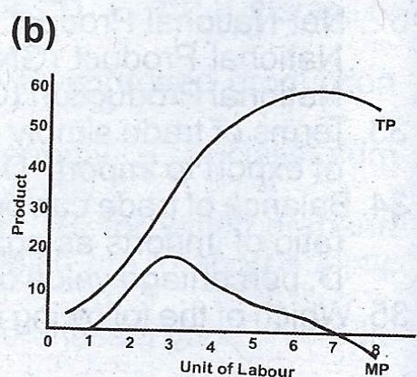
(c) Both TP and MP rise initially. The TP curve is at maxi-mum when MP is zero.
TP declines after MP = 0 and MP assumes negative values
At N6 = 400 - 150 = 250 units
(c) Excess supply at prices N8, N9 and N10 .
Excess supplied at N8 = 400 - 250 = 150 units
at N9 = 500 - 150 = 350units
at N10 = 600 - 50 =550 units
(d) At price N7, Quantity is 300 units


Contributions ({{ comment_count }})
Please wait...
Modal title
Report
Block User
{{ feedback_modal_data.title }}